(image) (image) [ Previous ] [ Home ] [ Next ]

Modeling Spin-Orbit Torques
in Advanced Magnetoresistive Devices

\(\newcommand{\footnotename}{footnote}\) \(\def \LWRfootnote {1}\) \(\newcommand {\footnote }[2][\LWRfootnote ]{{}^{\mathrm {#1}}}\) \(\newcommand {\footnotemark }[1][\LWRfootnote ]{{}^{\mathrm {#1}}}\) \(\let \LWRorighspace \hspace \) \(\renewcommand {\hspace }{\ifstar \LWRorighspace \LWRorighspace }\) \(\newcommand {\mathnormal }[1]{{#1}}\) \(\newcommand \ensuremath [1]{#1}\) \(\newcommand {\LWRframebox }[2][]{\fbox {#2}} \newcommand {\framebox }[1][]{\LWRframebox } \) \(\newcommand {\setlength }[2]{}\) \(\newcommand {\addtolength }[2]{}\) \(\newcommand {\setcounter }[2]{}\) \(\newcommand {\addtocounter }[2]{}\) \(\newcommand {\arabic }[1]{}\) \(\newcommand {\number }[1]{}\) \(\newcommand {\noalign }[1]{\text {#1}\notag \\}\) \(\newcommand {\cline }[1]{}\) \(\newcommand {\directlua }[1]{\text {(directlua)}}\) \(\newcommand {\luatexdirectlua }[1]{\text {(directlua)}}\) \(\newcommand {\protect }{}\) \(\def \LWRabsorbnumber #1 {}\) \(\def \LWRabsorbquotenumber "#1 {}\) \(\newcommand {\LWRabsorboption }[1][]{}\) \(\newcommand {\LWRabsorbtwooptions }[1][]{\LWRabsorboption }\) \(\def \mathchar {\ifnextchar "\LWRabsorbquotenumber \LWRabsorbnumber }\) \(\def \mathcode #1={\mathchar }\) \(\let \delcode \mathcode \) \(\let \delimiter \mathchar \) \(\def \oe {\unicode {x0153}}\) \(\def \OE {\unicode {x0152}}\) \(\def \ae {\unicode {x00E6}}\) \(\def \AE {\unicode {x00C6}}\) \(\def \aa {\unicode {x00E5}}\) \(\def \AA {\unicode {x00C5}}\) \(\def \o {\unicode {x00F8}}\) \(\def \O {\unicode {x00D8}}\) \(\def \l {\unicode {x0142}}\) \(\def \L {\unicode {x0141}}\) \(\def \ss {\unicode {x00DF}}\) \(\def \SS {\unicode {x1E9E}}\) \(\def \dag {\unicode {x2020}}\) \(\def \ddag {\unicode {x2021}}\) \(\def \P {\unicode {x00B6}}\) \(\def \copyright {\unicode {x00A9}}\) \(\def \pounds {\unicode {x00A3}}\) \(\let \LWRref \ref \) \(\renewcommand {\ref }{\ifstar \LWRref \LWRref }\) \( \newcommand {\multicolumn }[3]{#3}\) \(\require {textcomp}\) \(\newcommand {\mathlarger }[1]{#1}\) \(\newcommand {\mathsmaller }[1]{#1}\) \(\newcommand {\intertext }[1]{\text {#1}\notag \\}\) \(\let \Hat \hat \) \(\let \Check \check \) \(\let \Tilde \tilde \) \(\let \Acute \acute \) \(\let \Grave \grave \) \(\let \Dot \dot \) \(\let \Ddot \ddot \) \(\let \Breve \breve \) \(\let \Bar \bar \) \(\let \Vec \vec \) \(\newcommand {\bm }[1]{\boldsymbol {#1}}\) \(\require {mathtools}\) \(\newenvironment {crampedsubarray}[1]{}{}\) \(\newcommand {\smashoperator }[2][]{#2\limits }\) \(\newcommand {\SwapAboveDisplaySkip }{}\) \(\newcommand {\LaTeXunderbrace }[1]{\underbrace {#1}}\) \(\newcommand {\LaTeXoverbrace }[1]{\overbrace {#1}}\) \(\newcommand {\LWRmultlined }[1][]{\begin {multline*}}\) \(\newenvironment {multlined}[1][]{\LWRmultlined }{\end {multline*}}\) \(\let \LWRorigshoveleft \shoveleft \) \(\renewcommand {\shoveleft }[1][]{\LWRorigshoveleft }\) \(\let \LWRorigshoveright \shoveright \) \(\renewcommand {\shoveright }[1][]{\LWRorigshoveright }\) \(\newcommand {\shortintertext }[1]{\text {#1}\notag \\}\) \(\newcommand {\vcentcolon }{\mathrel {\unicode {x2236}}}\) \(\newcommand {\tothe }[1]{^{#1}}\) \(\newcommand {\raiseto }[2]{{#2}^{#1}}\) \(\newcommand {\LWRsiunitxEND }{}\) \(\def \LWRsiunitxang #1;#2;#3;#4\LWRsiunitxEND {\ifblank {#1}{}{\num {#1}\degree }\ifblank {#2}{}{\num {#2}^{\unicode {x2032}}}\ifblank {#3}{}{\num {#3}^{\unicode {x2033}}}}\) \(\newcommand {\ang }[2][]{\LWRsiunitxang #2;;;\LWRsiunitxEND }\) \(\def \LWRsiunitxdistribunit {}\) \(\newcommand {\LWRsiunitxENDTWO }{}\) \(\def \LWRsiunitxprintdecimalsubtwo #1,#2,#3\LWRsiunitxENDTWO {\ifblank {#1}{0}{\mathrm {#1}}\ifblank {#2}{}{{\LWRsiunitxdecimal }\mathrm {#2}}}\) \(\def \LWRsiunitxprintdecimalsub #1.#2.#3\LWRsiunitxEND {\LWRsiunitxprintdecimalsubtwo #1,,\LWRsiunitxENDTWO \ifblank {#2}{}{{\LWRsiunitxdecimal }\LWRsiunitxprintdecimalsubtwo #2,,\LWRsiunitxENDTWO }}\) \(\newcommand {\LWRsiunitxprintdecimal }[1]{\LWRsiunitxprintdecimalsub #1...\LWRsiunitxEND }\) \(\def \LWRsiunitxnumplus #1+#2+#3\LWRsiunitxEND {\ifblank {#2}{\LWRsiunitxprintdecimal {#1}}{\ifblank {#1}{\LWRsiunitxprintdecimal {#2}}{\LWRsiunitxprintdecimal {#1}\unicode {x02B}\LWRsiunitxprintdecimal {#2}}}\LWRsiunitxdistribunit }\) \(\def \LWRsiunitxnumminus #1-#2-#3\LWRsiunitxEND {\ifblank {#2}{\LWRsiunitxnumplus #1+++\LWRsiunitxEND }{\ifblank {#1}{}{\LWRsiunitxprintdecimal {#1}}\unicode {x02212}\LWRsiunitxprintdecimal {#2}\LWRsiunitxdistribunit }}\) \(\def \LWRsiunitxnumpmmacro #1\pm #2\pm #3\LWRsiunitxEND {\ifblank {#2}{\LWRsiunitxnumminus #1---\LWRsiunitxEND }{\LWRsiunitxprintdecimal {#1}\unicode {x0B1}\LWRsiunitxprintdecimal {#2}\LWRsiunitxdistribunit }}\) \(\def \LWRsiunitxnumpm #1+-#2+-#3\LWRsiunitxEND {\ifblank {#2}{\LWRsiunitxnumpmmacro #1\pm \pm \pm \LWRsiunitxEND }{\LWRsiunitxprintdecimal {#1}\unicode {x0B1}\LWRsiunitxprintdecimal {#2}\LWRsiunitxdistribunit }}\) \(\newcommand {\LWRsiunitxnumscientific }[2]{\ifblank {#1}{}{\ifstrequal {#1}{-}{-}{\LWRsiunitxprintdecimal {#1}\times }}10^{\LWRsiunitxprintdecimal {#2}}\LWRsiunitxdistribunit }\) \(\def \LWRsiunitxnumD #1D#2D#3\LWRsiunitxEND {\ifblank {#2}{\LWRsiunitxnumpm #1+-+-\LWRsiunitxEND }{\mathrm {\LWRsiunitxnumscientific {#1}{#2}}}}\) \(\def \LWRsiunitxnumd #1d#2d#3\LWRsiunitxEND {\ifblank {#2}{\LWRsiunitxnumD #1DDD\LWRsiunitxEND }{\mathrm {\LWRsiunitxnumscientific {#1}{#2}}}}\) \(\def \LWRsiunitxnumE #1E#2E#3\LWRsiunitxEND {\ifblank {#2}{\LWRsiunitxnumd #1ddd\LWRsiunitxEND }{\mathrm {\LWRsiunitxnumscientific {#1}{#2}}}}\) \(\def \LWRsiunitxnume #1e#2e#3\LWRsiunitxEND {\ifblank {#2}{\LWRsiunitxnumE #1EEE\LWRsiunitxEND }{\mathrm {\LWRsiunitxnumscientific {#1}{#2}}}}\) \(\def \LWRsiunitxnumx #1x#2x#3x#4\LWRsiunitxEND {\ifblank {#2}{\LWRsiunitxnume #1eee\LWRsiunitxEND }{\ifblank {#3}{\LWRsiunitxnume #1eee\LWRsiunitxEND \times \LWRsiunitxnume #2eee\LWRsiunitxEND }{\LWRsiunitxnume #1eee\LWRsiunitxEND \times \LWRsiunitxnume #2eee\LWRsiunitxEND \times \LWRsiunitxnume #3eee\LWRsiunitxEND }}}\) \(\newcommand {\num }[2][]{\LWRsiunitxnumx #2xxxxx\LWRsiunitxEND }\) \(\newcommand {\si }[2][]{\mathrm {\gsubstitute {#2}{~}{\,}}}\) \(\def \LWRsiunitxSIopt #1[#2]#3{\def \LWRsiunitxdistribunit {\,\si {#3}}{#2}\num {#1}\def \LWRsiunitxdistribunit {}}\) \(\newcommand {\LWRsiunitxSI }[2]{\def \LWRsiunitxdistribunit {\,\si {#2}}\num {#1}\def \LWRsiunitxdistribunit {}}\) \(\newcommand {\SI }[2][]{\ifnextchar [{\LWRsiunitxSIopt {#2}}{\LWRsiunitxSI {#2}}}\) \(\newcommand {\numlist }[2][]{\text {#2}}\) \(\newcommand {\numrange }[3][]{\num {#2}\ \LWRsiunitxrangephrase \ \num {#3}}\) \(\newcommand {\SIlist }[3][]{\text {#2}\,\si {#3}}\) \(\newcommand {\SIrange }[4][]{\num {#2}\,#4\ \LWRsiunitxrangephrase \ \num {#3}\,#4}\) \(\newcommand {\tablenum }[2][]{\mathrm {#2}}\) \(\newcommand {\ampere }{\mathrm {A}}\) \(\newcommand {\candela }{\mathrm {cd}}\) \(\newcommand {\kelvin }{\mathrm {K}}\) \(\newcommand {\kilogram }{\mathrm {kg}}\) \(\newcommand {\metre }{\mathrm {m}}\) \(\newcommand {\mole }{\mathrm {mol}}\) \(\newcommand {\second }{\mathrm {s}}\) \(\newcommand {\becquerel }{\mathrm {Bq}}\) \(\newcommand {\degreeCelsius }{\unicode {x2103}}\) \(\newcommand {\coulomb }{\mathrm {C}}\) \(\newcommand {\farad }{\mathrm {F}}\) \(\newcommand {\gray }{\mathrm {Gy}}\) \(\newcommand {\hertz }{\mathrm {Hz}}\) \(\newcommand {\henry }{\mathrm {H}}\) \(\newcommand {\joule }{\mathrm {J}}\) \(\newcommand {\katal }{\mathrm {kat}}\) \(\newcommand {\lumen }{\mathrm {lm}}\) \(\newcommand {\lux }{\mathrm {lx}}\) \(\newcommand {\newton }{\mathrm {N}}\) \(\newcommand {\ohm }{\mathrm {\Omega }}\) \(\newcommand {\pascal }{\mathrm {Pa}}\) \(\newcommand {\radian }{\mathrm {rad}}\) \(\newcommand {\siemens }{\mathrm {S}}\) \(\newcommand {\sievert }{\mathrm {Sv}}\) \(\newcommand {\steradian }{\mathrm {sr}}\) \(\newcommand {\tesla }{\mathrm {T}}\) \(\newcommand {\volt }{\mathrm {V}}\) \(\newcommand {\watt }{\mathrm {W}}\) \(\newcommand {\weber }{\mathrm {Wb}}\) \(\newcommand {\day }{\mathrm {d}}\) \(\newcommand {\degree }{\mathrm {^\circ }}\) \(\newcommand {\hectare }{\mathrm {ha}}\) \(\newcommand {\hour }{\mathrm {h}}\) \(\newcommand {\litre }{\mathrm {l}}\) \(\newcommand {\liter }{\mathrm {L}}\) \(\newcommand {\arcminute }{^\prime }\) \(\newcommand {\minute }{\mathrm {min}}\) \(\newcommand {\arcsecond }{^{\prime \prime }}\) \(\newcommand {\tonne }{\mathrm {t}}\) \(\newcommand {\astronomicalunit }{au}\) \(\newcommand {\atomicmassunit }{u}\) \(\newcommand {\bohr }{\mathit {a}_0}\) \(\newcommand {\clight }{\mathit {c}_0}\) \(\newcommand {\dalton }{\mathrm {D}_\mathrm {a}}\) \(\newcommand {\electronmass }{\mathit {m}_{\mathrm {e}}}\) \(\newcommand {\electronvolt }{\mathrm {eV}}\) \(\newcommand {\elementarycharge }{\mathit {e}}\) \(\newcommand {\hartree }{\mathit {E}_{\mathrm {h}}}\) \(\newcommand {\planckbar }{\mathit {\unicode {x210F}}}\) \(\newcommand {\angstrom }{\mathrm {\unicode {x212B}}}\) \(\let \LWRorigbar \bar \) \(\newcommand {\bar }{\mathrm {bar}}\) \(\newcommand {\barn }{\mathrm {b}}\) \(\newcommand {\bel }{\mathrm {B}}\) \(\newcommand {\decibel }{\mathrm {dB}}\) \(\newcommand {\knot }{\mathrm {kn}}\) \(\newcommand {\mmHg }{\mathrm {mmHg}}\) \(\newcommand {\nauticalmile }{\mathrm {M}}\) \(\newcommand {\neper }{\mathrm {Np}}\) \(\newcommand {\yocto }{\mathrm {y}}\) \(\newcommand {\zepto }{\mathrm {z}}\) \(\newcommand {\atto }{\mathrm {a}}\) \(\newcommand {\femto }{\mathrm {f}}\) \(\newcommand {\pico }{\mathrm {p}}\) \(\newcommand {\nano }{\mathrm {n}}\) \(\newcommand {\micro }{\mathrm {\unicode {x00B5}}}\) \(\newcommand {\milli }{\mathrm {m}}\) \(\newcommand {\centi }{\mathrm {c}}\) \(\newcommand {\deci }{\mathrm {d}}\) \(\newcommand {\deca }{\mathrm {da}}\) \(\newcommand {\hecto }{\mathrm {h}}\) \(\newcommand {\kilo }{\mathrm {k}}\) \(\newcommand {\mega }{\mathrm {M}}\) \(\newcommand {\giga }{\mathrm {G}}\) \(\newcommand {\tera }{\mathrm {T}}\) \(\newcommand {\peta }{\mathrm {P}}\) \(\newcommand {\exa }{\mathrm {E}}\) \(\newcommand {\zetta }{\mathrm {Z}}\) \(\newcommand {\yotta }{\mathrm {Y}}\) \(\newcommand {\percent }{\mathrm {\%}}\) \(\newcommand {\meter }{\mathrm {m}}\) \(\newcommand {\metre }{\mathrm {m}}\) \(\newcommand {\gram }{\mathrm {g}}\) \(\newcommand {\kg }{\kilo \gram }\) \(\newcommand {\of }[1]{_{\mathrm {#1}}}\) \(\newcommand {\squared }{^2}\) \(\newcommand {\square }[1]{\mathrm {#1}^2}\) \(\newcommand {\cubed }{^3}\) \(\newcommand {\cubic }[1]{\mathrm {#1}^3}\) \(\newcommand {\per }{\,\mathrm {/}}\) \(\newcommand {\celsius }{\unicode {x2103}}\) \(\newcommand {\fg }{\femto \gram }\) \(\newcommand {\pg }{\pico \gram }\) \(\newcommand {\ng }{\nano \gram }\) \(\newcommand {\ug }{\micro \gram }\) \(\newcommand {\mg }{\milli \gram }\) \(\newcommand {\g }{\gram }\) \(\newcommand {\kg }{\kilo \gram }\) \(\newcommand {\amu }{\mathrm {u}}\) \(\newcommand {\pm }{\pico \metre }\) \(\newcommand {\nm }{\nano \metre }\) \(\newcommand {\um }{\micro \metre }\) \(\newcommand {\mm }{\milli \metre }\) \(\newcommand {\cm }{\centi \metre }\) \(\newcommand {\dm }{\deci \metre }\) \(\newcommand {\m }{\metre }\) \(\newcommand {\km }{\kilo \metre }\) \(\newcommand {\as }{\atto \second }\) \(\newcommand {\fs }{\femto \second }\) \(\newcommand {\ps }{\pico \second }\) \(\newcommand {\ns }{\nano \second }\) \(\newcommand {\us }{\micro \second }\) \(\newcommand {\ms }{\milli \second }\) \(\newcommand {\s }{\second }\) \(\newcommand {\fmol }{\femto \mol }\) \(\newcommand {\pmol }{\pico \mol }\) \(\newcommand {\nmol }{\nano \mol }\) \(\newcommand {\umol }{\micro \mol }\) \(\newcommand {\mmol }{\milli \mol }\) \(\newcommand {\mol }{\mol }\) \(\newcommand {\kmol }{\kilo \mol }\) \(\newcommand {\pA }{\pico \ampere }\) \(\newcommand {\nA }{\nano \ampere }\) \(\newcommand {\uA }{\micro \ampere }\) \(\newcommand {\mA }{\milli \ampere }\) \(\newcommand {\A }{\ampere }\) \(\newcommand {\kA }{\kilo \ampere }\) \(\newcommand {\ul }{\micro \litre }\) \(\newcommand {\ml }{\milli \litre }\) \(\newcommand {\l }{\litre }\) \(\newcommand {\hl }{\hecto \litre }\) \(\newcommand {\uL }{\micro \liter }\) \(\newcommand {\mL }{\milli \liter }\) \(\newcommand {\L }{\liter }\) \(\newcommand {\hL }{\hecto \liter }\) \(\newcommand {\mHz }{\milli \hertz }\) \(\newcommand {\Hz }{\hertz }\) \(\newcommand {\kHz }{\kilo \hertz }\) \(\newcommand {\MHz }{\mega \hertz }\) \(\newcommand {\GHz }{\giga \hertz }\) \(\newcommand {\THz }{\tera \hertz }\) \(\newcommand {\mN }{\milli \newton }\) \(\newcommand {\N }{\newton }\) \(\newcommand {\kN }{\kilo \newton }\) \(\newcommand {\MN }{\mega \newton }\) \(\newcommand {\Pa }{\pascal }\) \(\newcommand {\kPa }{\kilo \pascal }\) \(\newcommand {\MPa }{\mega \pascal }\) \(\newcommand {\GPa }{\giga \pascal }\) \(\newcommand {\mohm }{\milli \ohm }\) \(\newcommand {\kohm }{\kilo \ohm }\) \(\newcommand {\Mohm }{\mega \ohm }\) \(\newcommand {\pV }{\pico \volt }\) \(\newcommand {\nV }{\nano \volt }\) \(\newcommand {\uV }{\micro \volt }\) \(\newcommand {\mV }{\milli \volt }\) \(\newcommand {\V }{\volt }\) \(\newcommand {\kV }{\kilo \volt }\) \(\newcommand {\W }{\watt }\) \(\newcommand {\uW }{\micro \watt }\) \(\newcommand {\mW }{\milli \watt }\) \(\newcommand {\kW }{\kilo \watt }\) \(\newcommand {\MW }{\mega \watt }\) \(\newcommand {\GW }{\giga \watt }\) \(\newcommand {\J }{\joule }\) \(\newcommand {\uJ }{\micro \joule }\) \(\newcommand {\mJ }{\milli \joule }\) \(\newcommand {\kJ }{\kilo \joule }\) \(\newcommand {\eV }{\electronvolt }\) \(\newcommand {\meV }{\milli \electronvolt }\) \(\newcommand {\keV }{\kilo \electronvolt }\) \(\newcommand {\MeV }{\mega \electronvolt }\) \(\newcommand {\GeV }{\giga \electronvolt }\) \(\newcommand {\TeV }{\tera \electronvolt }\) \(\newcommand {\kWh }{\kilo \watt \hour }\) \(\newcommand {\F }{\farad }\) \(\newcommand {\fF }{\femto \farad }\) \(\newcommand {\pF }{\pico \farad }\) \(\newcommand {\K }{\mathrm {K}}\) \(\newcommand {\dB }{\mathrm {dB}}\) \(\newcommand {\kibi }{\mathrm {Ki}}\) \(\newcommand {\mebi }{\mathrm {Mi}}\) \(\newcommand {\gibi }{\mathrm {Gi}}\) \(\newcommand {\tebi }{\mathrm {Ti}}\) \(\newcommand {\pebi }{\mathrm {Pi}}\) \(\newcommand {\exbi }{\mathrm {Ei}}\) \(\newcommand {\zebi }{\mathrm {Zi}}\) \(\newcommand {\yobi }{\mathrm {Yi}}\) \(\let \unit \si \) \(\let \qty \SI \) \(\let \qtylist \SIlist \) \(\let \qtyrange \SIrange \) \(\let \numproduct \num \) \(\let \qtyproduct \SI \) \(\let \complexnum \num \) \(\newcommand {\complexqty }[3][]{(\complexnum {#2})\si {#3}}\) \(\def \LWRsiunitxrangephrase {\TextOrMath { }{\ }\protect \mbox {to}\TextOrMath { }{\ }}\) \(\def \LWRsiunitxdecimal {.}\)

7.3 Angular Dependence of SOTs

Thus far, the torques have only been discussed in terms of the FL and DL components, with the well-established magnetization dependence:

\begin{align} \bm {\tau _\mathrm {FL}} & = \tau _\mathrm {FL}\bm {m}\times \bm {p}, \\ \bm {\tau _\mathrm {DL}} & = \tau _\mathrm {DL}\bm {m}\times \left (\bm {m}\times \bm {p}\right ), \end{align} where \(\bm {p}\) is the polarization direction of the spin accumulation, and \(\tau _\mathrm {FL}\) and \(\tau _\mathrm {DL}\) are the constant magnitudes of the FL and DL torques, respectively. For CIP NM/FM bilayers with the FL torque is predominantly attributed to the REE, while the DL torque is primarily attributed to the SHE, both generating a spin polarization along \(\bm {p} = \bm {E}\times \bm {\hat {z}}\).

Most descriptions of SOT in CIP bilayers only account for the conventional DL and FL torques. However, the symmetry of the bilayer system allows for a more complicated dependence on the magnetization direction, which has been confirmed by experiments and ab initio calculations [113, 114, 115]:

\begin{equation} \bm {\tau } = \sum ^\infty _{l=0} (m_z)^{2l} \left \{a_l\bm {m}\times (\bm {E}\times \bm {\hat {z}}) + b_l\bm {m}\times [\bm {m}\times (\bm {E}\times \bm {\hat {z}})] + c_l(\bm {m}\cdot \bm {E})\bm {m}\times \bm {\hat {z}} + d_l(\bm {m}\cdot \bm {E})[\bm {m}\times (\bm {m}\times \bm {\hat {z}})]\right \}, \end{equation}

where \(a_l\), \(b_l\), \(c_l\) and \(d_l\), are expansion coefficients. For \(l=0\), the first two terms represent the typical DL and FL torques. The last two terms are new contributions that vanish when the magnetization is perpendicular to the applied electric field. These additional contributions are referred to as higher-order SOTs. Previous models based on the REE effect in 2D FM systems have accounted for the strong dependence on the magnetization direction [116, 117], showing that the angular dependence appears when the SOC and exchange coupling are comparable in strength.

In this section, the angular dependence of the SOTs in CIP NM/FM bilayers is investigated using the 1D-CSDD model and the IMR-BCs derived in chapter 5. The perturbation theory SOC model is only valid in the weak SOC regime and only accounts for the typical FL and DL terms. Extending the perturbation theory to higher orders in SOC could perhaps capture these contributions; however, this is left for future work. Nonetheless, since the effective interface field model is valid in the strong SOC regime, it will be used in this section to model the interface. The results and discussions in the following two subsections were adapted from work published in Scientific Reports at the time of writing [79].

7.3.1 Higher-Order SOTs

(image)

Figure 7.12: A schematic of a NM/FM bilayer system with an electric field \(\bm {E}\) applied along \(x\). The magnetization direction of the FM layer \(\bm {m}\) is described by the polar and azimuthal angles \(\theta \) and \(\phi \), respectively. The figure was published in Ref. [79].

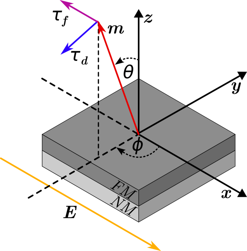
The CIP NM/FM bilayer system considered is depicted in Fig. 7.12, where the in-plane electric field is along \(x\), and the magnetization is described by the polar and azimuthal angles \(\theta \) and \(\phi \), respectively, thus the magnetization direction can be expressed as

\begin{equation} \bm {m} = [\cos (\phi )\sin (\theta ), \sin (\phi )\sin (\theta ),\cos (\theta )]. \end{equation}

When \(\phi = 0^\circ \), the DL torque reduces to

\begin{equation} \bm {\tau _\mathrm {DL}}(\bm {m}) = \tau _\mathrm {DL}(\bm {m}) \, \bm {\hat {y}}, \end{equation}

and for \(\phi = 90^\circ \), the FL torque becomes

\begin{equation} \bm {\tau _\mathrm {FL}}(\bm {m}) = \tau _\mathrm {FL}(\bm {m}) \cos (\theta ) \, \bm {\hat {x}}. \end{equation}

By varying the polar angle \(\theta \) in each plane, the angular dependence of the DL and FL torque magnitudes \(\tau _\mathrm {DL}(\bm {m})\) and \(\tau _\mathrm {FL}(\bm {m})\), respectively, can be analyzed. To determine the total torque acting on the magnetization, the 1D-CSDD model is solved for the bilayer system.

Material parameters for Pt and Co are selected for the NM and FM layers, respectively, and are summarized in Table 7.4. To determine suitable interfacial parameters, the calculated torques are fitted to experimental measurements reported for a Pt(\(3\,\si {nm}\))/Co(\(0.6\,\si {nm}\))/AlO\(_x\)(\(1.6\,\si {nm}\)) trilayer system [113]. The resistivity of the full stack was measured to be \(36\,\si {\micro \ohm \centi \meter }\), for a device width of \(1\,\si {\micro \meter }\) carrying a current of \(1.136\,\si {\milli \ampere }\), Ohm’s law gives an applied electric field of \(7.86\,\si {\mega \volt \per \meter }\). The torques are computed using this estimated electric field together with the bulk conductivities of Pt and Co listed in Table 7.4. As AlO\(_x\) is an insulator, it is not included in the calculations. For direct comparison with the experimental values, the units of the calculated total torque are converted from A/s to T by multiplying with \(1/(\gamma M_s d_{F})\), where \(d_{F}\) is the FM thickness. For Pt/Co systems, the saturation magnetization of Co is taken as \(M_s \approx 600\,\si {\kilo \ampere \per \meter }\) [118].

(image)

Figure 7.13: Computed and measured SOTs for two different CIP NM/FM bilayer systems as a function of the polar angle of the magnetization. The system considered is illustrated in Fig. 7.12, where the magnetization direction is described in terms of polar (\(\theta \)) and azimuthal angles (\(\phi \)). Column (a,c): the FL torque for \(\phi = 90^\circ \); column (b,d): the DL torque for \(\phi = 0^\circ \); row (a- b): Pt (3 nm)/Co (0.6 nm) bilayer system; row (c-d): Ta (3 nm)/CoFeB (0.9 nm) bilayer system. The computed torques were obtained using the bulk and interface parameters listed in Tables 7.4 and 7.5, respectively. The figure was adapted from reference [79].

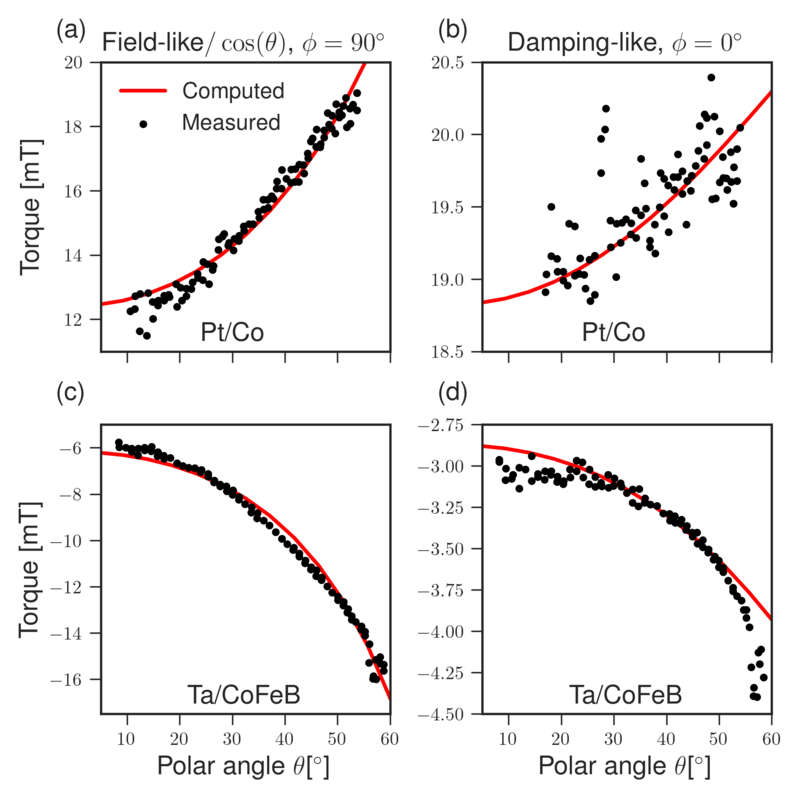
The best fit obtained by setting \(k_F = 16 \,\si {nm^{-1}}\) and treating \(u_0\), \(u_m\), and \(u_R\) as fitting parameters is shown in Fig. 7.13a,b. The parameter values were fitted using the nonlinear least-squares method, and are listed in Table 7.5. The fitted FL and DL torque magnitudes show excellent agreement with the experimental data, confirming that the model successfully captures both the strong FL torque and the higher-order torque contributions reported in previous studies. The FL torque magnitude exhibits a pronounced angular dependence, whereas the angular variation of the DL torque magnitude is comparatively weaker.

.
Parameter Pt Ta Co CoFeB Units
\(\sigma \) \(7\,\)[102] \(0.5\,\)[119] \(5\,\)[104] \(3.3\,\)[103] \(\mathrm {MSm^{-1}}\)
\(\alpha _\mathrm {SH}\) \(0.19\)[102] \(-0.15\,\)[40] 1
\(\beta _\sigma ,\beta _D\) \(0.36\,\)[104] \(0.56\,\)[103] 1
\(\lambda _\mathrm {sf}\) \(1.4\,\)[102] \(1.9\,\)[119] \(38\,\)[104] \(12\,\)[104, 103] nm
\(\lambda _{J}\) \(1.2\,\)[120] \(1.2\,\)[120] nm
\(\lambda _{\phi }\) \(1.8\,\)[120, 63] \(2.0\,\) nm
Table 7.4: Material parameters taken from reported values in the literature or extracted from experimental or ab initio data. For Co, the dephasing length (\(\lambda _\phi \)) was computed from the exchange length (\(\lambda _J\)) reported by Ghosh et al. [120], using the coherence (\(l_\perp \)) and precession lengths (\(l_L\)) extracted by Petitjean et al. [63], from the ab initio data reported by Brataas et al. [65]. For CoFeB, the spin-flip length was obtained from the experimental data reported by Oshima et al. [103], using equation (18) from Piraux et al. [104].
.
Parameter Pt/Co Ta/CoFeB Units
\(u_0\) \(0.06\) \(0.07\) 1
\(u_m\) \(0.28\) \(1.56\) 1
\(u_R\) \(0.22\) \(-1.18\) 1
\(k_F\) \(16\) \(15\) nm\(^{-1}\)
\(\tau ^\mathrm {F}\) \(1.28\) \(1.04\) fs
\(\tau ^\mathrm {N}\) \(1.80\) \(1.56\) fs
Table 7.5: Interface parameters obtained by fitting the angular dependence of the computed torques with the experimental data from Garello et al. [113]. The momentum relaxation times were computed from the bulk conductivities in Tab. 7.4 together with the Fermi wavenumber using the Drude model.

Experimental measurements of the angular dependence were also reported for a Ta(\(3.0\,\si {nm}\))/CoFeB(\(0.9\,\si {nm}\)) bilayer with a MgO(\(2.0\,\si {nm}\)) capping layer [113]. For this system, the resistivity was measured as \(184\,\si {\micro \ohm \centi \meter }\), and with a current of \(500\,\si {\micro \ampere }\) applied to a sample of width \(1\,\si {\micro \meter }\), the in-plane electric field is estimated to be \(15.7\,\si {\mega \volt \per \meter }\). Figure 7.13c,d presents the best fit obtained using the bulk and interface parameters summarized in Tables 7.4 and 7.5, respectively, together with a CoFeB saturation magnetization of \(M_s \approx 810\,\si {\kilo \ampere \per \meter }\) [121]. The fit reproduces the experimental data well, except for the DL torque at both small and large polar angles. In this system, the FL torque dominates and shows a strong angular dependence. Unlike the Pt/Co system, both torque components appear with opposite sign, consistent with the negative spin Hall angle of Ta and the fitted Rashba SOC magnitude.

For both the Pt/Co and Ta/CoFeB systems, the additional interfaces introduced by the insulating capping layer and the substrate (SiO\(_2\)) in the experimental setup were not included in the model. However, it has been shown that the choice of substrate can significantly influence current-induced torques when the NM layer is thin [122], suggesting that the substrate interface may also act as a source of spin currents. Similarly, the FM/oxide capping interface can also generate spin currents [123]. Both effects could contribute to the experimental results reported in [113], possibly accounting for the discrepancies observed in the Ta/CoFeB fits. Additionally, the model assumes flat and sharp interfaces, thereby neglecting interfacial roughness and intermixing.

Roughness enhances incoherent spin scattering and introduces spatial variations in the Rashba spin-orbit field, thereby reducing interface transparency and lowering the overall spin torque efficiency. On the other hand, scattering due to roughness could in principle generate weak spin currents, analogous to the spin Hall currents caused by impurity scattering in the bulk [124]. Intermixing results in a finite-thickness interfacial region with transport properties that differ from those of the adjacent bulk layers. Such a mixed region can strengthen the interfacial SOC, simultaneously enhancing the SOTs and increasing spin-memory loss [125, 126]. A relatively thick intermixed region has indeed been reported for the Ta/CoFeB interface [127], in clear disagreement with the assumptions of an idealized sharp interface. Finally, strain at the interfaces could further modify the SOC and associated SOTs. For example, in zinc-blende structures, the bulk Dresselhaus SOC acquires a modified form in the presence of interfacial strain [128].

Although interface disorder and strain can have a significant impact on SOTs, their effect on the angular dependence remains unclear due to the limited number of experimental studies on this subject. Annealing, however, has been shown to modify both the magnitude and angular dependence of the torques. In Ta/CoFeB bilayers, a marked increase in the angular dependence of the DL torque was observed once the annealing temperature exceeded \(270^\circ \mathrm {C}\) [129]. Since higher annealing temperatures are known to broaden the intermixing region at the Ta/CoFeB interface [130], this suggests that a thick intermixed interface may account for the discrepancy between the fitted and measured angular dependence of the DL torque in the Ta/CoFeB system, as the experimental data were obtained at \(300^\circ \mathrm {C}\). In principle, modeling the interface as a finite-thickness potential barrier within the Hamiltonian could capture the effects of intermixing; however, this is beyond the scope of the present work and is left for future investigations. Nevertheless, the strong agreement between the torques obtained with this interface model and the experimental data provides compelling evidence for an interfacial Rashba-type SOC at both Pt/Co and Ta/CoFeB interfaces.

7.3.2 Modification of SOTs by Interfacial Rashba
Spin-Orbit Coupling

(image)

Figure 7.14: The spin torque as a function of the polar angle of the magnetization for different strengths of the: Rashba SOC \(u_R\) (a-b), magnetic exchange interaction \(u_m\) (c-d). The parameters for the Co/Pt system presented in Table 7.4 and 7.5 were used for the computation. The figure was adapted from reference [79].

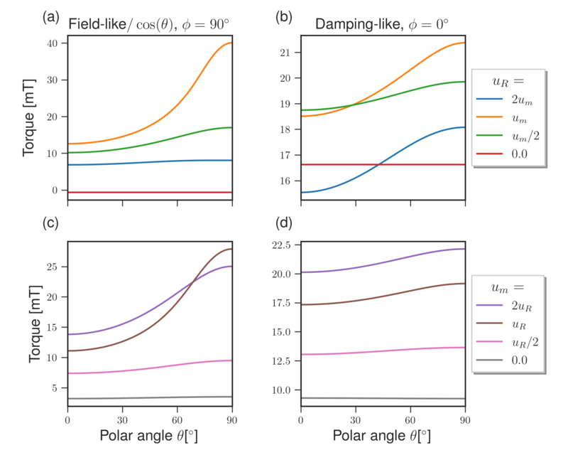
To examine the respective roles of Rashba SOC and the magnetic exchange interaction at the interface, the angular dependence of the SOTs is calculated for different values of \(u_R\) and \(u_m\) using the Co/Pt parameters from the previous section. The resulting SOTs are shown in Fig. 7.14. Both the FL and DL torques exhibit a strong dependence on the interaction strengths. The FL torque displays the largest magnitude and most pronounced angular variation when the interfacial SOC and magnetic exchange interactions are comparable. For either stronger or weaker relative interaction strengths, both the angular dependence and the magnitude are reduced. The DL torque exhibits a similar trend, but reaches its maximum when \(u_m > u_R\). In the limiting cases where either \(u_R = 0\) or \(u_m = 0\), the angular dependence of both FL and DL torques vanishes.

Similar results have been reported using 2D free electron and tight-binding models when both Rashba and magnetic exchange interactions are included [117]. In those studies, the angular dependence was attributed to the deformation of the Fermi surface spin texture when the Rashba and exchange interactions are of comparable strength. An intrinsic contribution from the Fermi sea to the DL torque was also identified. The 3D scattering model employed here differs substantially from such 2D approaches. In this model, only the electrons scattering off the effective field at the interface and the resulting outbound currents are considered. By contrast, 2D models treat the interface itself as the entire system, considering only the electrons within it and neglecting the interface scattering of bulk electrons. Within the interface scattering model, the effect of Fermi surface deformation is implicitly captured through the strong momentum dependence of the majority/minority potential barriers \(u^{\uparrow /\downarrow }_{\bm {k}}\) and the spin-projection operators \(\hat {p}^{\uparrow /\downarrow }_{\bm {k}}\) when \(u_R\) and \(u_m\) are of comparable magnitude. However, the intrinsic Fermi-sea contribution is not included, as it arises from modifications of the electronic wave function induced by the applied electric field, which is not considered in this model. Nevertheless, the scattering approach is more applicable to bilayer interfaces due to being 3D, thus allowing for additional effects due to in-plane and out-of-plane spin and charge currents on either side of the interface interacting with the SOC to be accounted for.

(image)

Figure 7.15: The spin torque as a function of the Rashba SOC strength (a-b) and the polar angle of the magnetization (c-d) showing the different contributions to the total torque. Column (a,c): the FL torque for \(\phi = 90^\circ \); column (b,d): the DL torque for \(\phi = 0^\circ \). For (a-b): \(\theta = 0\), and the dashed line marks \(u_R = u_m\). The parameters for the Pt/Co system presented in Table 7.4 and 7.5 were used for the computation. The figure was adapted from reference [79].

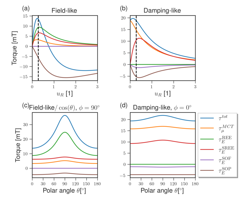
The individual contributions to the total spin torque captured by the 3D scattering model as a function of the Rashba interaction strength \(u_R\) are shown in Fig. 7.15a-b. As expected, in the limit of vanishing SOC, the additional in-plane current contributions disappear, leaving only the MCT contribution from the bulk SHE-generated spin accumulation. In contrast to conventional 2D REE models and the perturbation theory approach, the in-plane current contributions in this model do not scale linearly with \(u_R\). Instead, most contributions reach a maximum near \(u_R \approx u_m\) (except the SOP) and subsequently decrease in magnitude as \(u_R\) increases. The reduction originates from the increased lattice torque at the interface, which consistently reduces the MCT contribution \(\tau _\mu ^{\mathrm {MCT}}\) through spin-memory loss of the incident SHE current with increasing \(u_R\). The SOC-driven contributions initially grow with \(u_R\) as in-plane currents are more efficiently converted into out-of-plane spin currents. They reach their maximum near \(u_R \approx u_m\), where interfacial precession around the magnetization most effectively generates transverse spin components. For larger \(u_R\), the lattice torque begins to dominate, while transmission is strongly suppressed and reflection is enhanced as the potential barrier surpasses the Fermi energy. Consequently, the SOP contribution, which relies only on spin-dependent reflections, dominates the FL torque for \(u_R > u_m\) and peaks near \(u_R \approx 1.5u_m\). The decomposition further shows that the SOF contributes exclusively to the DL torque, while the SOP contributes to both DL and FL torques, with both terms opposing the other torque contributions. Consistent with 2D models, the REE produces only a FL torque; however, the SREE contributes to both components and constitutes the dominant contribution to the DL torque aside from the MCT term. Figures 7.15c-d illustrate the angular dependence of the different torque terms, which exhibit qualitatively similar trends with varying strength. In particular, the REE is found to be primarily responsible for the strong angular dependence of the FL torque magnitude, while the MCT torque also acquires an angular dependence through SOC-induced modifications.