(image) (image) [ Previous ] [ Home ] [ Next ]

Modeling Spin-Orbit Torques
in Advanced Magnetoresistive Devices

\(\newcommand{\footnotename}{footnote}\) \(\def \LWRfootnote {1}\) \(\newcommand {\footnote }[2][\LWRfootnote ]{{}^{\mathrm {#1}}}\) \(\newcommand {\footnotemark }[1][\LWRfootnote ]{{}^{\mathrm {#1}}}\) \(\let \LWRorighspace \hspace \) \(\renewcommand {\hspace }{\ifstar \LWRorighspace \LWRorighspace }\) \(\newcommand {\mathnormal }[1]{{#1}}\) \(\newcommand \ensuremath [1]{#1}\) \(\newcommand {\LWRframebox }[2][]{\fbox {#2}} \newcommand {\framebox }[1][]{\LWRframebox } \) \(\newcommand {\setlength }[2]{}\) \(\newcommand {\addtolength }[2]{}\) \(\newcommand {\setcounter }[2]{}\) \(\newcommand {\addtocounter }[2]{}\) \(\newcommand {\arabic }[1]{}\) \(\newcommand {\number }[1]{}\) \(\newcommand {\noalign }[1]{\text {#1}\notag \\}\) \(\newcommand {\cline }[1]{}\) \(\newcommand {\directlua }[1]{\text {(directlua)}}\) \(\newcommand {\luatexdirectlua }[1]{\text {(directlua)}}\) \(\newcommand {\protect }{}\) \(\def \LWRabsorbnumber #1 {}\) \(\def \LWRabsorbquotenumber "#1 {}\) \(\newcommand {\LWRabsorboption }[1][]{}\) \(\newcommand {\LWRabsorbtwooptions }[1][]{\LWRabsorboption }\) \(\def \mathchar {\ifnextchar "\LWRabsorbquotenumber \LWRabsorbnumber }\) \(\def \mathcode #1={\mathchar }\) \(\let \delcode \mathcode \) \(\let \delimiter \mathchar \) \(\def \oe {\unicode {x0153}}\) \(\def \OE {\unicode {x0152}}\) \(\def \ae {\unicode {x00E6}}\) \(\def \AE {\unicode {x00C6}}\) \(\def \aa {\unicode {x00E5}}\) \(\def \AA {\unicode {x00C5}}\) \(\def \o {\unicode {x00F8}}\) \(\def \O {\unicode {x00D8}}\) \(\def \l {\unicode {x0142}}\) \(\def \L {\unicode {x0141}}\) \(\def \ss {\unicode {x00DF}}\) \(\def \SS {\unicode {x1E9E}}\) \(\def \dag {\unicode {x2020}}\) \(\def \ddag {\unicode {x2021}}\) \(\def \P {\unicode {x00B6}}\) \(\def \copyright {\unicode {x00A9}}\) \(\def \pounds {\unicode {x00A3}}\) \(\let \LWRref \ref \) \(\renewcommand {\ref }{\ifstar \LWRref \LWRref }\) \( \newcommand {\multicolumn }[3]{#3}\) \(\require {textcomp}\) \(\newcommand {\mathlarger }[1]{#1}\) \(\newcommand {\mathsmaller }[1]{#1}\) \(\newcommand {\intertext }[1]{\text {#1}\notag \\}\) \(\let \Hat \hat \) \(\let \Check \check \) \(\let \Tilde \tilde \) \(\let \Acute \acute \) \(\let \Grave \grave \) \(\let \Dot \dot \) \(\let \Ddot \ddot \) \(\let \Breve \breve \) \(\let \Bar \bar \) \(\let \Vec \vec \) \(\newcommand {\bm }[1]{\boldsymbol {#1}}\) \(\require {mathtools}\) \(\newenvironment {crampedsubarray}[1]{}{}\) \(\newcommand {\smashoperator }[2][]{#2\limits }\) \(\newcommand {\SwapAboveDisplaySkip }{}\) \(\newcommand {\LaTeXunderbrace }[1]{\underbrace {#1}}\) \(\newcommand {\LaTeXoverbrace }[1]{\overbrace {#1}}\) \(\newcommand {\LWRmultlined }[1][]{\begin {multline*}}\) \(\newenvironment {multlined}[1][]{\LWRmultlined }{\end {multline*}}\) \(\let \LWRorigshoveleft \shoveleft \) \(\renewcommand {\shoveleft }[1][]{\LWRorigshoveleft }\) \(\let \LWRorigshoveright \shoveright \) \(\renewcommand {\shoveright }[1][]{\LWRorigshoveright }\) \(\newcommand {\shortintertext }[1]{\text {#1}\notag \\}\) \(\newcommand {\vcentcolon }{\mathrel {\unicode {x2236}}}\) \(\newcommand {\tothe }[1]{^{#1}}\) \(\newcommand {\raiseto }[2]{{#2}^{#1}}\) \(\newcommand {\LWRsiunitxEND }{}\) \(\def \LWRsiunitxang #1;#2;#3;#4\LWRsiunitxEND {\ifblank {#1}{}{\num {#1}\degree }\ifblank {#2}{}{\num {#2}^{\unicode {x2032}}}\ifblank {#3}{}{\num {#3}^{\unicode {x2033}}}}\) \(\newcommand {\ang }[2][]{\LWRsiunitxang #2;;;\LWRsiunitxEND }\) \(\def \LWRsiunitxdistribunit {}\) \(\newcommand {\LWRsiunitxENDTWO }{}\) \(\def \LWRsiunitxprintdecimalsubtwo #1,#2,#3\LWRsiunitxENDTWO {\ifblank {#1}{0}{\mathrm {#1}}\ifblank {#2}{}{{\LWRsiunitxdecimal }\mathrm {#2}}}\) \(\def \LWRsiunitxprintdecimalsub #1.#2.#3\LWRsiunitxEND {\LWRsiunitxprintdecimalsubtwo #1,,\LWRsiunitxENDTWO \ifblank {#2}{}{{\LWRsiunitxdecimal }\LWRsiunitxprintdecimalsubtwo #2,,\LWRsiunitxENDTWO }}\) \(\newcommand {\LWRsiunitxprintdecimal }[1]{\LWRsiunitxprintdecimalsub #1...\LWRsiunitxEND }\) \(\def \LWRsiunitxnumplus #1+#2+#3\LWRsiunitxEND {\ifblank {#2}{\LWRsiunitxprintdecimal {#1}}{\ifblank {#1}{\LWRsiunitxprintdecimal {#2}}{\LWRsiunitxprintdecimal {#1}\unicode {x02B}\LWRsiunitxprintdecimal {#2}}}\LWRsiunitxdistribunit }\) \(\def \LWRsiunitxnumminus #1-#2-#3\LWRsiunitxEND {\ifblank {#2}{\LWRsiunitxnumplus #1+++\LWRsiunitxEND }{\ifblank {#1}{}{\LWRsiunitxprintdecimal {#1}}\unicode {x02212}\LWRsiunitxprintdecimal {#2}\LWRsiunitxdistribunit }}\) \(\def \LWRsiunitxnumpmmacro #1\pm #2\pm #3\LWRsiunitxEND {\ifblank {#2}{\LWRsiunitxnumminus #1---\LWRsiunitxEND }{\LWRsiunitxprintdecimal {#1}\unicode {x0B1}\LWRsiunitxprintdecimal {#2}\LWRsiunitxdistribunit }}\) \(\def \LWRsiunitxnumpm #1+-#2+-#3\LWRsiunitxEND {\ifblank {#2}{\LWRsiunitxnumpmmacro #1\pm \pm \pm \LWRsiunitxEND }{\LWRsiunitxprintdecimal {#1}\unicode {x0B1}\LWRsiunitxprintdecimal {#2}\LWRsiunitxdistribunit }}\) \(\newcommand {\LWRsiunitxnumscientific }[2]{\ifblank {#1}{}{\ifstrequal {#1}{-}{-}{\LWRsiunitxprintdecimal {#1}\times }}10^{\LWRsiunitxprintdecimal {#2}}\LWRsiunitxdistribunit }\) \(\def \LWRsiunitxnumD #1D#2D#3\LWRsiunitxEND {\ifblank {#2}{\LWRsiunitxnumpm #1+-+-\LWRsiunitxEND }{\mathrm {\LWRsiunitxnumscientific {#1}{#2}}}}\) \(\def \LWRsiunitxnumd #1d#2d#3\LWRsiunitxEND {\ifblank {#2}{\LWRsiunitxnumD #1DDD\LWRsiunitxEND }{\mathrm {\LWRsiunitxnumscientific {#1}{#2}}}}\) \(\def \LWRsiunitxnumE #1E#2E#3\LWRsiunitxEND {\ifblank {#2}{\LWRsiunitxnumd #1ddd\LWRsiunitxEND }{\mathrm {\LWRsiunitxnumscientific {#1}{#2}}}}\) \(\def \LWRsiunitxnume #1e#2e#3\LWRsiunitxEND {\ifblank {#2}{\LWRsiunitxnumE #1EEE\LWRsiunitxEND }{\mathrm {\LWRsiunitxnumscientific {#1}{#2}}}}\) \(\def \LWRsiunitxnumx #1x#2x#3x#4\LWRsiunitxEND {\ifblank {#2}{\LWRsiunitxnume #1eee\LWRsiunitxEND }{\ifblank {#3}{\LWRsiunitxnume #1eee\LWRsiunitxEND \times \LWRsiunitxnume #2eee\LWRsiunitxEND }{\LWRsiunitxnume #1eee\LWRsiunitxEND \times \LWRsiunitxnume #2eee\LWRsiunitxEND \times \LWRsiunitxnume #3eee\LWRsiunitxEND }}}\) \(\newcommand {\num }[2][]{\LWRsiunitxnumx #2xxxxx\LWRsiunitxEND }\) \(\newcommand {\si }[2][]{\mathrm {\gsubstitute {#2}{~}{\,}}}\) \(\def \LWRsiunitxSIopt #1[#2]#3{\def \LWRsiunitxdistribunit {\,\si {#3}}{#2}\num {#1}\def \LWRsiunitxdistribunit {}}\) \(\newcommand {\LWRsiunitxSI }[2]{\def \LWRsiunitxdistribunit {\,\si {#2}}\num {#1}\def \LWRsiunitxdistribunit {}}\) \(\newcommand {\SI }[2][]{\ifnextchar [{\LWRsiunitxSIopt {#2}}{\LWRsiunitxSI {#2}}}\) \(\newcommand {\numlist }[2][]{\text {#2}}\) \(\newcommand {\numrange }[3][]{\num {#2}\ \LWRsiunitxrangephrase \ \num {#3}}\) \(\newcommand {\SIlist }[3][]{\text {#2}\,\si {#3}}\) \(\newcommand {\SIrange }[4][]{\num {#2}\,#4\ \LWRsiunitxrangephrase \ \num {#3}\,#4}\) \(\newcommand {\tablenum }[2][]{\mathrm {#2}}\) \(\newcommand {\ampere }{\mathrm {A}}\) \(\newcommand {\candela }{\mathrm {cd}}\) \(\newcommand {\kelvin }{\mathrm {K}}\) \(\newcommand {\kilogram }{\mathrm {kg}}\) \(\newcommand {\metre }{\mathrm {m}}\) \(\newcommand {\mole }{\mathrm {mol}}\) \(\newcommand {\second }{\mathrm {s}}\) \(\newcommand {\becquerel }{\mathrm {Bq}}\) \(\newcommand {\degreeCelsius }{\unicode {x2103}}\) \(\newcommand {\coulomb }{\mathrm {C}}\) \(\newcommand {\farad }{\mathrm {F}}\) \(\newcommand {\gray }{\mathrm {Gy}}\) \(\newcommand {\hertz }{\mathrm {Hz}}\) \(\newcommand {\henry }{\mathrm {H}}\) \(\newcommand {\joule }{\mathrm {J}}\) \(\newcommand {\katal }{\mathrm {kat}}\) \(\newcommand {\lumen }{\mathrm {lm}}\) \(\newcommand {\lux }{\mathrm {lx}}\) \(\newcommand {\newton }{\mathrm {N}}\) \(\newcommand {\ohm }{\mathrm {\Omega }}\) \(\newcommand {\pascal }{\mathrm {Pa}}\) \(\newcommand {\radian }{\mathrm {rad}}\) \(\newcommand {\siemens }{\mathrm {S}}\) \(\newcommand {\sievert }{\mathrm {Sv}}\) \(\newcommand {\steradian }{\mathrm {sr}}\) \(\newcommand {\tesla }{\mathrm {T}}\) \(\newcommand {\volt }{\mathrm {V}}\) \(\newcommand {\watt }{\mathrm {W}}\) \(\newcommand {\weber }{\mathrm {Wb}}\) \(\newcommand {\day }{\mathrm {d}}\) \(\newcommand {\degree }{\mathrm {^\circ }}\) \(\newcommand {\hectare }{\mathrm {ha}}\) \(\newcommand {\hour }{\mathrm {h}}\) \(\newcommand {\litre }{\mathrm {l}}\) \(\newcommand {\liter }{\mathrm {L}}\) \(\newcommand {\arcminute }{^\prime }\) \(\newcommand {\minute }{\mathrm {min}}\) \(\newcommand {\arcsecond }{^{\prime \prime }}\) \(\newcommand {\tonne }{\mathrm {t}}\) \(\newcommand {\astronomicalunit }{au}\) \(\newcommand {\atomicmassunit }{u}\) \(\newcommand {\bohr }{\mathit {a}_0}\) \(\newcommand {\clight }{\mathit {c}_0}\) \(\newcommand {\dalton }{\mathrm {D}_\mathrm {a}}\) \(\newcommand {\electronmass }{\mathit {m}_{\mathrm {e}}}\) \(\newcommand {\electronvolt }{\mathrm {eV}}\) \(\newcommand {\elementarycharge }{\mathit {e}}\) \(\newcommand {\hartree }{\mathit {E}_{\mathrm {h}}}\) \(\newcommand {\planckbar }{\mathit {\unicode {x210F}}}\) \(\newcommand {\angstrom }{\mathrm {\unicode {x212B}}}\) \(\let \LWRorigbar \bar \) \(\newcommand {\bar }{\mathrm {bar}}\) \(\newcommand {\barn }{\mathrm {b}}\) \(\newcommand {\bel }{\mathrm {B}}\) \(\newcommand {\decibel }{\mathrm {dB}}\) \(\newcommand {\knot }{\mathrm {kn}}\) \(\newcommand {\mmHg }{\mathrm {mmHg}}\) \(\newcommand {\nauticalmile }{\mathrm {M}}\) \(\newcommand {\neper }{\mathrm {Np}}\) \(\newcommand {\yocto }{\mathrm {y}}\) \(\newcommand {\zepto }{\mathrm {z}}\) \(\newcommand {\atto }{\mathrm {a}}\) \(\newcommand {\femto }{\mathrm {f}}\) \(\newcommand {\pico }{\mathrm {p}}\) \(\newcommand {\nano }{\mathrm {n}}\) \(\newcommand {\micro }{\mathrm {\unicode {x00B5}}}\) \(\newcommand {\milli }{\mathrm {m}}\) \(\newcommand {\centi }{\mathrm {c}}\) \(\newcommand {\deci }{\mathrm {d}}\) \(\newcommand {\deca }{\mathrm {da}}\) \(\newcommand {\hecto }{\mathrm {h}}\) \(\newcommand {\kilo }{\mathrm {k}}\) \(\newcommand {\mega }{\mathrm {M}}\) \(\newcommand {\giga }{\mathrm {G}}\) \(\newcommand {\tera }{\mathrm {T}}\) \(\newcommand {\peta }{\mathrm {P}}\) \(\newcommand {\exa }{\mathrm {E}}\) \(\newcommand {\zetta }{\mathrm {Z}}\) \(\newcommand {\yotta }{\mathrm {Y}}\) \(\newcommand {\percent }{\mathrm {\%}}\) \(\newcommand {\meter }{\mathrm {m}}\) \(\newcommand {\metre }{\mathrm {m}}\) \(\newcommand {\gram }{\mathrm {g}}\) \(\newcommand {\kg }{\kilo \gram }\) \(\newcommand {\of }[1]{_{\mathrm {#1}}}\) \(\newcommand {\squared }{^2}\) \(\newcommand {\square }[1]{\mathrm {#1}^2}\) \(\newcommand {\cubed }{^3}\) \(\newcommand {\cubic }[1]{\mathrm {#1}^3}\) \(\newcommand {\per }{\,\mathrm {/}}\) \(\newcommand {\celsius }{\unicode {x2103}}\) \(\newcommand {\fg }{\femto \gram }\) \(\newcommand {\pg }{\pico \gram }\) \(\newcommand {\ng }{\nano \gram }\) \(\newcommand {\ug }{\micro \gram }\) \(\newcommand {\mg }{\milli \gram }\) \(\newcommand {\g }{\gram }\) \(\newcommand {\kg }{\kilo \gram }\) \(\newcommand {\amu }{\mathrm {u}}\) \(\newcommand {\pm }{\pico \metre }\) \(\newcommand {\nm }{\nano \metre }\) \(\newcommand {\um }{\micro \metre }\) \(\newcommand {\mm }{\milli \metre }\) \(\newcommand {\cm }{\centi \metre }\) \(\newcommand {\dm }{\deci \metre }\) \(\newcommand {\m }{\metre }\) \(\newcommand {\km }{\kilo \metre }\) \(\newcommand {\as }{\atto \second }\) \(\newcommand {\fs }{\femto \second }\) \(\newcommand {\ps }{\pico \second }\) \(\newcommand {\ns }{\nano \second }\) \(\newcommand {\us }{\micro \second }\) \(\newcommand {\ms }{\milli \second }\) \(\newcommand {\s }{\second }\) \(\newcommand {\fmol }{\femto \mol }\) \(\newcommand {\pmol }{\pico \mol }\) \(\newcommand {\nmol }{\nano \mol }\) \(\newcommand {\umol }{\micro \mol }\) \(\newcommand {\mmol }{\milli \mol }\) \(\newcommand {\mol }{\mol }\) \(\newcommand {\kmol }{\kilo \mol }\) \(\newcommand {\pA }{\pico \ampere }\) \(\newcommand {\nA }{\nano \ampere }\) \(\newcommand {\uA }{\micro \ampere }\) \(\newcommand {\mA }{\milli \ampere }\) \(\newcommand {\A }{\ampere }\) \(\newcommand {\kA }{\kilo \ampere }\) \(\newcommand {\ul }{\micro \litre }\) \(\newcommand {\ml }{\milli \litre }\) \(\newcommand {\l }{\litre }\) \(\newcommand {\hl }{\hecto \litre }\) \(\newcommand {\uL }{\micro \liter }\) \(\newcommand {\mL }{\milli \liter }\) \(\newcommand {\L }{\liter }\) \(\newcommand {\hL }{\hecto \liter }\) \(\newcommand {\mHz }{\milli \hertz }\) \(\newcommand {\Hz }{\hertz }\) \(\newcommand {\kHz }{\kilo \hertz }\) \(\newcommand {\MHz }{\mega \hertz }\) \(\newcommand {\GHz }{\giga \hertz }\) \(\newcommand {\THz }{\tera \hertz }\) \(\newcommand {\mN }{\milli \newton }\) \(\newcommand {\N }{\newton }\) \(\newcommand {\kN }{\kilo \newton }\) \(\newcommand {\MN }{\mega \newton }\) \(\newcommand {\Pa }{\pascal }\) \(\newcommand {\kPa }{\kilo \pascal }\) \(\newcommand {\MPa }{\mega \pascal }\) \(\newcommand {\GPa }{\giga \pascal }\) \(\newcommand {\mohm }{\milli \ohm }\) \(\newcommand {\kohm }{\kilo \ohm }\) \(\newcommand {\Mohm }{\mega \ohm }\) \(\newcommand {\pV }{\pico \volt }\) \(\newcommand {\nV }{\nano \volt }\) \(\newcommand {\uV }{\micro \volt }\) \(\newcommand {\mV }{\milli \volt }\) \(\newcommand {\V }{\volt }\) \(\newcommand {\kV }{\kilo \volt }\) \(\newcommand {\W }{\watt }\) \(\newcommand {\uW }{\micro \watt }\) \(\newcommand {\mW }{\milli \watt }\) \(\newcommand {\kW }{\kilo \watt }\) \(\newcommand {\MW }{\mega \watt }\) \(\newcommand {\GW }{\giga \watt }\) \(\newcommand {\J }{\joule }\) \(\newcommand {\uJ }{\micro \joule }\) \(\newcommand {\mJ }{\milli \joule }\) \(\newcommand {\kJ }{\kilo \joule }\) \(\newcommand {\eV }{\electronvolt }\) \(\newcommand {\meV }{\milli \electronvolt }\) \(\newcommand {\keV }{\kilo \electronvolt }\) \(\newcommand {\MeV }{\mega \electronvolt }\) \(\newcommand {\GeV }{\giga \electronvolt }\) \(\newcommand {\TeV }{\tera \electronvolt }\) \(\newcommand {\kWh }{\kilo \watt \hour }\) \(\newcommand {\F }{\farad }\) \(\newcommand {\fF }{\femto \farad }\) \(\newcommand {\pF }{\pico \farad }\) \(\newcommand {\K }{\mathrm {K}}\) \(\newcommand {\dB }{\mathrm {dB}}\) \(\newcommand {\kibi }{\mathrm {Ki}}\) \(\newcommand {\mebi }{\mathrm {Mi}}\) \(\newcommand {\gibi }{\mathrm {Gi}}\) \(\newcommand {\tebi }{\mathrm {Ti}}\) \(\newcommand {\pebi }{\mathrm {Pi}}\) \(\newcommand {\exbi }{\mathrm {Ei}}\) \(\newcommand {\zebi }{\mathrm {Zi}}\) \(\newcommand {\yobi }{\mathrm {Yi}}\) \(\let \unit \si \) \(\let \qty \SI \) \(\let \qtylist \SIlist \) \(\let \qtyrange \SIrange \) \(\let \numproduct \num \) \(\let \qtyproduct \SI \) \(\let \complexnum \num \) \(\newcommand {\complexqty }[3][]{(\complexnum {#2})\si {#3}}\) \(\def \LWRsiunitxrangephrase {\TextOrMath { }{\ }\protect \mbox {to}\TextOrMath { }{\ }}\) \(\def \LWRsiunitxdecimal {.}\)

Chapter 7 SOTs in Ferromagnetic Systems

In this chapter, the spin transport and SOTs in NM/FM bilayer and FM/NM/FM trilayer systems are analyzed using the computational methods presented in the previous chapter. First, the distribution of spin currents, accumulation, and torques in NM/FM bilayers is studied, followed by an examination of the thickness dependence and then the angular dependence of SOTs. Finally, the spin currents in FM/NM/FM trilayers are investigated along with the resulting unconventional SOTs. In the 1D cases, the interface normals of the layers point along the \(z\)-axis, and the current flow is along the \(x\)-axis.

7.1 Spin Currents, Accumulation and Torques

In this section, the SHE and RE are investigated in NM/FM bilayer systems using the spin drift-diffusion model with the BCs derived in chapter 5. The results are obtained using both the FEM solver and the 1D-CSDD solver. The FEM solver is used to compute the full spatial distribution of the spin accumulation and spin torque in 3D geometries, while the 1D-CSDD solver is used to compute the distribution in highly idealized 1D geometries, allowing for a more in-depth investigation of the effects of various parameters and BCs.

7.1.1 SHE in a Nonmagnetic Wire

(image)

(a) Cylindrical wire.
   

(image)

(b) Rectangular wire.
Figure 7.1: Spin accumulation generated by the SHE in a cylindrical (a) and rectangular (b) wire. The results were obtained with the FEM solver using the NM layer parameters from Table 6.1 with an applied electric field of \(10^{6}\,\mathrm {V/m}\) along the \(x\)-direction.

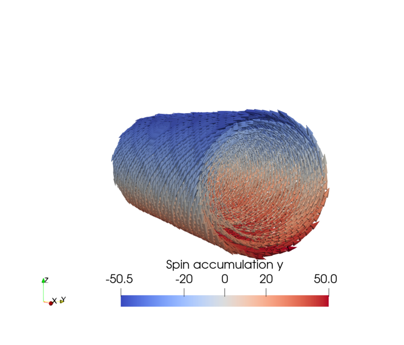
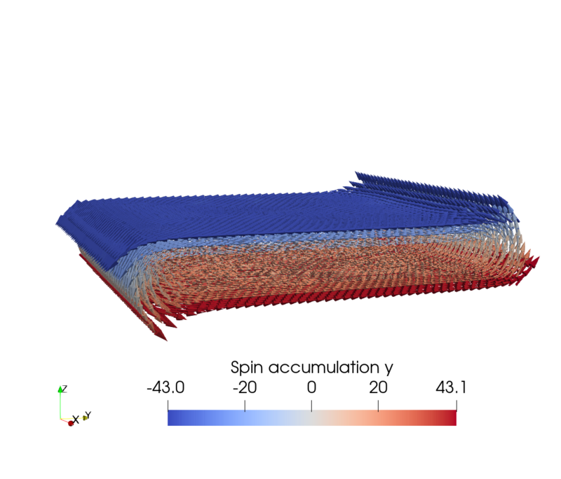
Considering a NM wire with an in-plane electric field, the SHE generates a spin accumulation at the interface of the wire with a polarization perpendicular to the current and the interface normal. Figure 7.1 shows the spin accumulation generated by the SHE in a cylindrical and rectangular wire, respectively, computed with the FEM solver using the parameters presented in Table 6.1 with an applied electric field of \(10^{6}\,\mathrm {V/m}\) along the \(x\)-direction. The cylindrical wire has a radius of \(10\,\mathrm {nm}\) and the rectangular wire has a width of \(60\,\mathrm {nm}\) and a thickness of \(10\,\mathrm {nm}\). As expected, the polarization direction of the spin accumulation at the boundary is described by the cross product \(\bm {\hat {p}} = \bm {\hat {E}}\times \bm {n}\), where \(\bm {n}\) is the interface normal. Thus, in the cylindrical wire, the spin accumulation wraps around the outer edges of the wire, whereas in the rectangular wire, it is uniformly aligned along the long sides and changes direction around the edges. In both cases, the spin accumulation at the upper part of the boundary of the wire is polarized along \(-y\).

(image)

Figure 7.2: Spin accumulation and spin current density generated by the SHE in a \(10\,\mathrm {nm}\) thick layer for various spin-flip lengths. The results were obtained with the 1D-CSDD solver using the NM layer parameters from Table 6.1 with a \(10^{6}\,\mathrm {V/m}\) applied electric field along the \(x\)-direction.

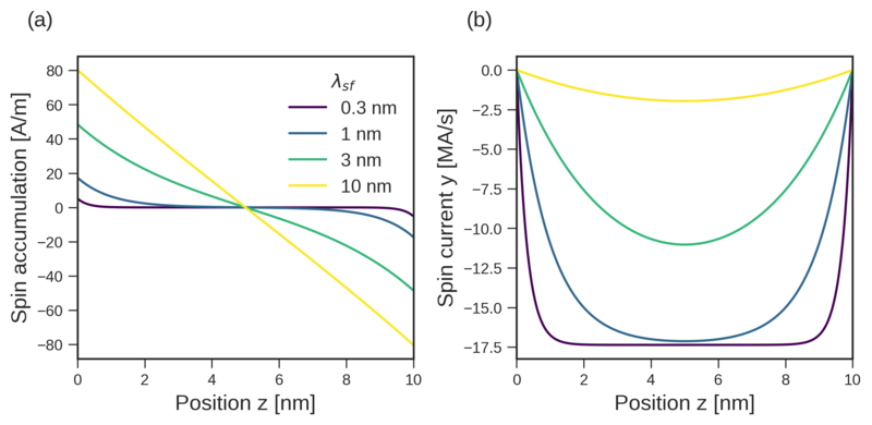
Assuming the length and width of the rectangular wire are much larger than the thickness, the drift-diffusion equations can be simplified to a 1D problem. Figure 7.2 shows the spin accumulation and spin current density generated by the SHE, computed with the 1D-CSDD solver for various spin-flip lengths. For longer spin-flip lengths, less of the net spin density generated in the bulk is lost to spin-flip scattering before reaching the boundary. Thus, longer spin-flip lengths result in an increasing build-up of spin accumulation at the boundary of the wire. At the boundary, the spin current is reflected, resulting in a diffusion spin current flowing back into the bulk, opposing the SHE-generated spin current. The reflected spin current penetrates deeper into the bulk for longer spin-flip lengths, resulting in a larger region where the net spin current is reduced. The distribution of the spin accumulation shows qualitatively good agreement with the first reported experimental observation of the SHE in GaAs [37].

7.1.2 SHE in Nonmagnetic/Ferromagnetic Bilayers

(image)

(a)

(image)

(b)

(image)

(c)
Figure 7.3: The normalized magnetization (a), spin accumulation generated by the SHE (b), and the resulting spin torque acting on the magnetization (c), in a NM/FM bilayer system. The results were computed using the FEM solver with the bulk and interface parameters from Table 6.1, except \(\lambda _\phi = 0.8\,\mathrm {nm}\), and a \(10^{6}\,\mathrm {V/m}\) electric field along the \(x\)-direction.

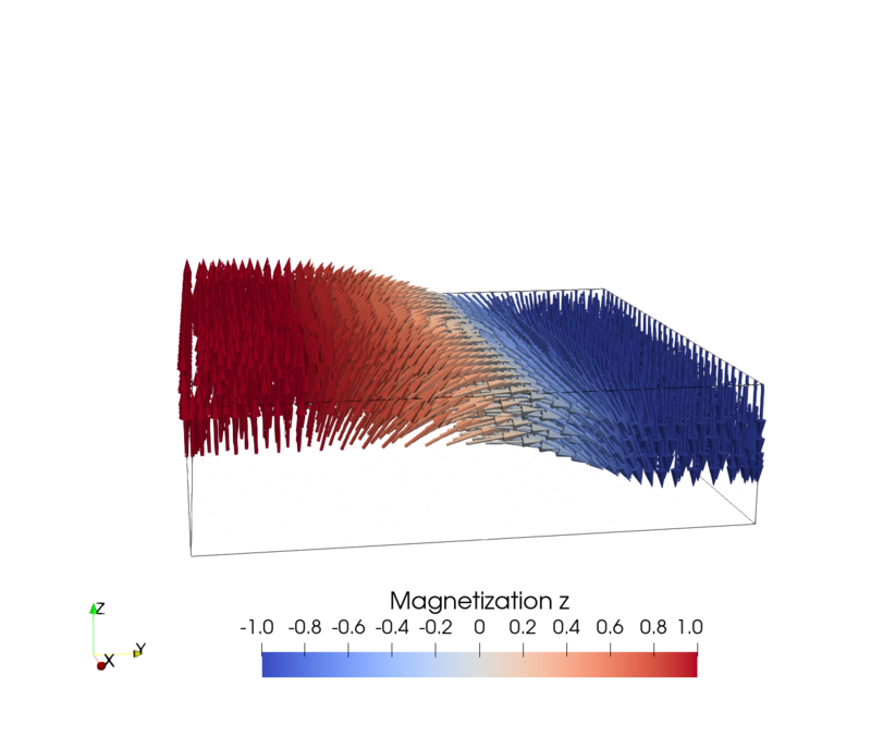
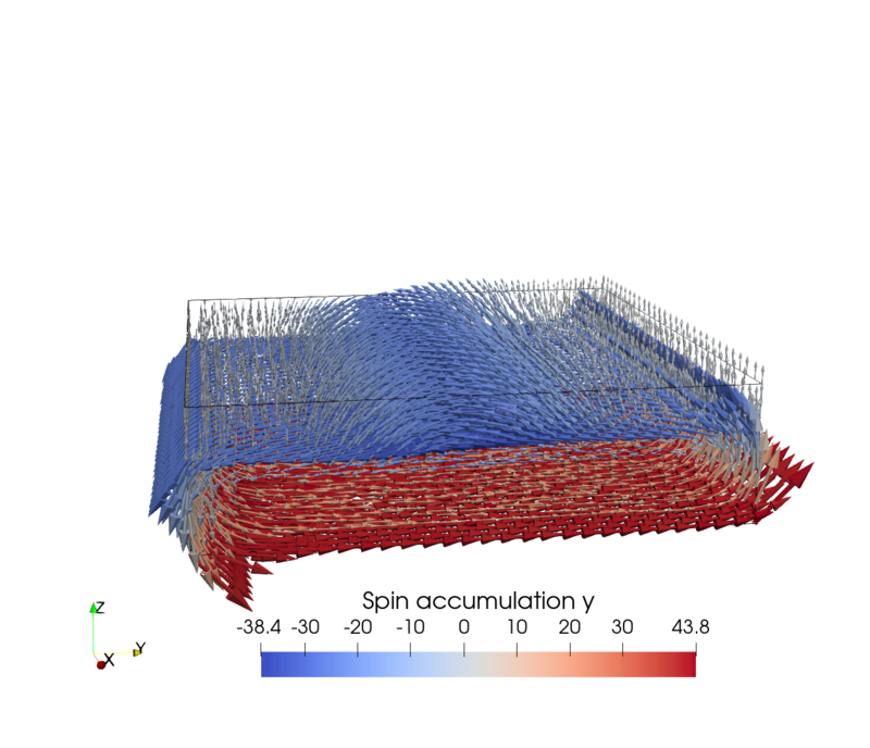
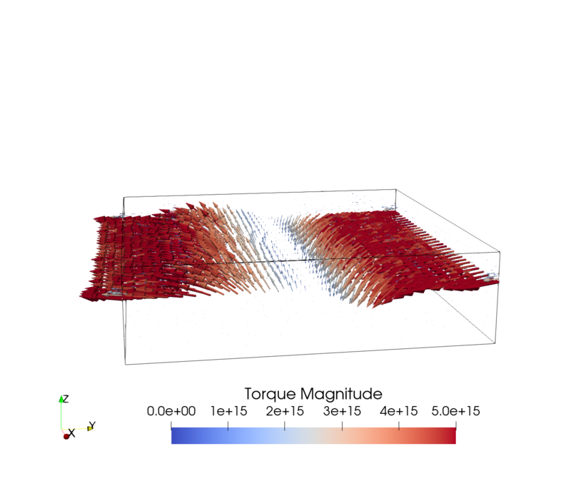
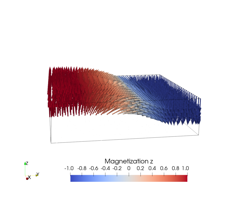
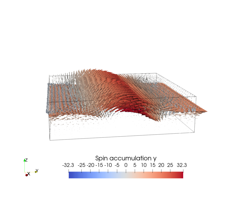
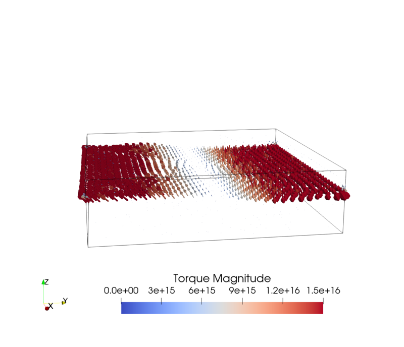
Placing a \(5\,\mathrm {nm}\) FM layer on top of the rectangular wire from Fig. 7.1b allows the spin accumulation at the upper boundary of the NM wire to leak into the FM, where the transverse spin angular momentum is transferred to the magnetization, resulting in spin torques. Figure 7.3 shows the distribution of the magnetization, the spin accumulation, and spin torque in the bilayer structure; interfacial SOC is omitted for now. The magnetization of the FM layer changes gradually its direction from \(+z\) to \(-z\) across a \(40\,\mathrm {nm}\) wide region in the middle of the FM, thus forming a Néel domain wall. When the magnetization is along \({\mathbin {\textpm }} z\), the spin accumulation generated by the SHE is transverse to the magnetization and decays quickly due to the short spin dephasing length. When the magnetization is in-plane, the spin accumulation is longitudinal and can penetrate deeper into the FM layer. The resulting torques are predominantly DL and are localized within a few nanometers from the interface, as expected from the short spin dephasing length.

.
Parameter Value Unit
\(u_0\) \(0.42645\) 1
\(u_m\) \(0.20055\) 1
\(u_R\) \(0.04\) 1
\(\tau _F\) \(6.00881\) fs
\(\tau _N\) \(1.12579\) fs
\(k_F\) \(16 \) nm\(^{-1}\)
Table 7.1: The interface parameters used to compute the BCs for the NM/FM interface taken from [70]. The majority and minority momentum relaxation times are given by \(\tau ^{\uparrow /\downarrow } = \tau _F {\mathbin {\textpm }} P\tau _F\), where \(P = \beta _\sigma \).

(image)

Figure 7.4: The distribution of the spin accumulation (a-b), spin current density (c-d), and spin torque (e-f) generated by the SHE in a NM/FM bilayer system. The results were obtained using the 1D-CSDD solver with the parame- ters presented in Table 6.1, except \(\lambda ^F_{sf} = 3\,\mathrm {nm}\) and \(\lambda _\phi = 0.8\,\mathrm {nm}\). The columns show results obtained us- ing different BCs at the NM/FM interface: IM-BCs (a, c, e), and MCT-BCs (b, d, f). The IM-BCs were computed using the interface parameters presented in Table 

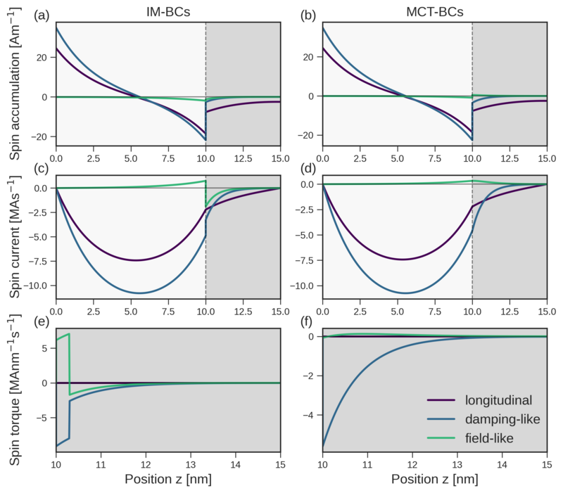
In the case of vanishing interfacial SOC (\(u_R = 0\)) the NM/FM interface can be treated using two different sets of BCs: the BCs from the MCT (MCT-BCs) presented in Eq. (4.35), and the interface magnetism BCs (IM-BCs) obtained by treating the interface as a spin-dependent delta function potential barrier with an interfacial magnetic exchange interaction, which are presented in Eq. (5.48). Fig 7.4 shows the results obtained with the 1D-CSDD solver for the spin accumulation, spin current density, and spin torque generated by the SHE in a NM/FM bilayer system using the two different BCs.

For the MCT-BCS, the spin currents are kept continuous across the interface and are related to the spin and charge potential drops through the interface conductances. In contrast, the IM-BCs allow for the spin current to be discontinuous across the interface by introducing a transmission mixing conductance, thereby capturing the absorption of transverse spin current due to the exchange interaction at the interface. The solutions are projected along the DL, FL, and longitudinal directions. The magnetization is oriented along \((1,1,1)\) such that all the components are non-zero, and the spin-flip length in the FM is set to \(3\,\mathrm {nm}\) to highlight the decay of the longitudinal component. To visualize the interface torque, it is included as a step function in the FM layer in the vicinity of the interface.

In both cases, the spin accumulation and spin current generated in the NM layer leak into the FM layer, where the transverse components quickly decay, resulting in a torque acting on the magnetization. The results obtained with the two BCs agree well in the NM layer; however, in the FM layer, they differ significantly. With the IM-BCs, the DL spin current is partially lost at the interface, resulting in a strong interfacial DL torque. Conversely, the FL spin current changes sign across the interface, causing the FL torque to act in the opposite direction at the interface compared to the bulk. For the MCT-BCs, the spin current is continuous across the interface, resulting in a torque acting on the magnetization only in the bulk of the FM layer. In both cases, the FL spin components are weak compared to the DL components, and appear at the interface as they are generated by the spin-dependent reflection captured by the imaginary part of the spin-mixing conductance and transmission spin-mixing conductance.

7.1.3 Rashba Effect in Nonmagnetic/Ferromagnetic
Bilayers

The RE is expected to play an important role in generating current-induced SOTs in NM/FM bilayers. Using the models derived in chapter 5, the effects of an interfacial Rashba SOC on the spin accumulation and torque in a NM/FM bilayer system are investigated. To focus on the RE, the SHE is omitted by setting \(\alpha _\mathrm {SH} = 0\). For the FEM results, the MCT-BCs, combined with the BCs treating the interfacial Rashba SOC using perturbation theory (IRPT-BCs), as presented in Eq. (5.25), are utilized due to their lower computational complexity. To later compare with the BCs based on the combined interfacial magnetic exchange and Rashba SOC interactions (IMR-BCs), presented in Eq. (5.34), the IRPT-BCs are computed using the same scattering matrices and parameters. The resulting analytical expressions for the interface conductances and conductivities are presented in Appendix A.

(image)

(a)

(image)

(b)

(image)

(c)
Figure 7.5: The same as Fig. 7.3 except with an interfacial Rashba SOC and without SHE (\(\alpha _\mathrm {SH} = 0\)). The Rashba SOC is treated using the IRPT-BCs. The Rashba interface conductivities are calculated using the analytical expressions presented in Appendix A with the parameters presented in Table 7.1.

The spin accumulation and torque obtained from considering a Rashba SOC at the interface of the NM/FM bilayer system from the previous section are shown in Fig. 7.5. In contrast to the SHE, the spin accumulation generated by the Rashba SOC originates from the interface instead of in the bulk and is not present at the outer boundaries. The spin accumulation is mostly polarized along \(y\), as expected for the REE. When the spin accumulation is transverse to the magnetization, it is quickly absorbed in the FM, while when it is longitudinal, it can penetrate deeper into the FM layer. As expected, the resulting torque has a strong FL component; however, a weaker DL component is also present. As the spin-flip length is significantly shorter in the NM layer compared to the FM layer, the spin accumulation decays more quickly away from the interface in the NM, whereas in the FM, it is more pronounced.

(image)

Figure 7.6: Same as Fig. 7.4 except with an interfacial Rashba SOC and \(\alpha _\mathrm {SH} = 0\). Column (a, c, e): results obtained with the IMR-BCs. Column (b, d, f): results obtained with the IRPT-BCs. The BCs were calculated using the parameters presented in Table 7.1.

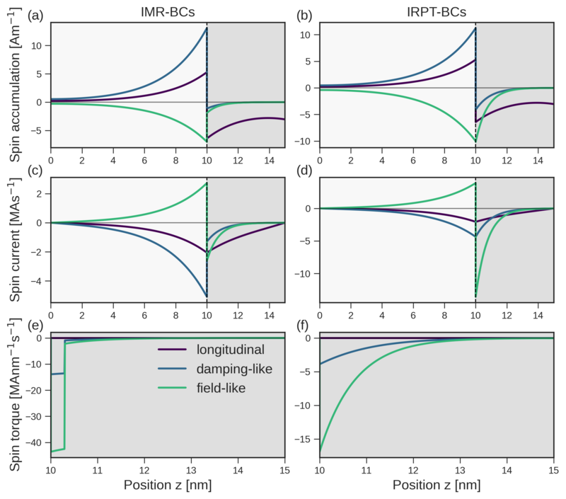
Fig 7.4 shows the spin accumulation, spin current density, and spin torque obtained with the 1D-CSDD solver for the Rashba SOC in the bilayer system using the two different sets of BCs. The two approaches agree well in the NM layer; however, they differ significantly in the FM layer. In both cases, both longitudinal and FL components of the spin accumulation and spin current are generated at the interface. With the IMR-BCs, both transverse spin current components are discontinuous across the interface, and the torque is primarily interfacial. With the IRPT-BCs, the FL spin current component is discontinuous across the interface, while the DL component is continuous; the resulting torque only acts in the bulk of the FM layer. In both cases, the FL components are strong compared to the DL components, in agreement with previous REE models.

7.1.4 Validity of the Perturbation Theory Approach to
Interfacial Rashba Spin-Orbit Coupling

(image)

Figure 7.7: The total spin torque generated by the interfacial Rashba SOC in a NM/FM bilayer as a function of the coupling strength \(u_R\) for various interfacial exchange interaction strengths \(u_m\). The same system and parameters as in Fig. 7.6 were used. The solid lines show the results obtained with the IMR-BCs, while the dashed lines show the results obtained using the IRPT-BCs.

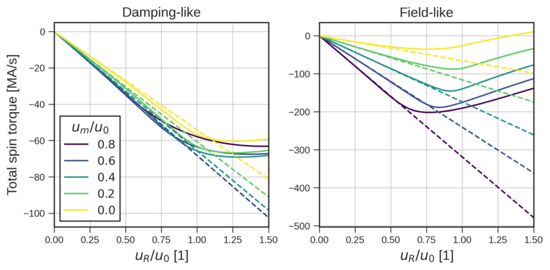
The IRPT-BCs assume that the Rashba SOC is small compared to other interactions, allowing it to be treated as a perturbation of the wave function. Consequently, these boundary conditions are expected to break down for large Rashba coupling strengths. To assess the validity range of this perturbative approach, the total spin torque acting on the magnetization in the bilayer system is computed for increasing \(u_R\). The total torque is obtained by integrating the torque density over the FM layer and dividing by its thickness. Figure 7.7 presents the resulting torques computed with the 1D-CSDD solver using both the IMR-BCs and IRPT-BCs.

For the IRPT-BCs, the FL torque is, in general, larger than the DL torque for all the values of \(u_R\) and \(u_m\) considered. Since the interface conductivities and torkivities obtained with the perturbation theory approach are first order in the Rashba SOC, the resulting torques are linear functions of \(u_R\). The slope of both the torque components increases with increased exchange interaction strength \(u_m\), which is strongly pronounced for the FL torque, while the DL torque is only slightly affected.

The torques obtained using the IMR-BCs exhibit a linear behavior only for small \(u_R\), approximately when \(u_R / u_0 < 0.5\), where both approaches show good agreement. For larger \(u_R\), the results deviate significantly, indicating that higher-order terms become relevant, which are not included in the first-order approximation of the perturbation theory. Both the DL and FL torques reach a maximum and subsequently decrease for larger \(u_R\).